16: Machine Learning with Scipy

Scipy contains very powerful modules for machine learning, data analysis, time series, etc. This notebook shows you some of the most useful functions

import numpy as np
import matplotlib.pyplot as plt

1) Interpolation

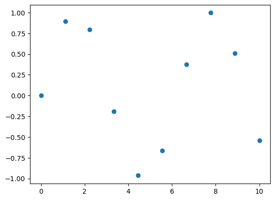
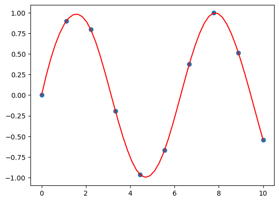
Interpolating a signal is sometimes very useful if you are missing data in a Dataset. But it is a dangerous technique, which can sometimes transform the reality of things!

# Dataset Creation
x = np.linspace(0, 10, 10)
y = np.sin(x)
plt.scatter(x, y)

<matplotlib.collections.PathCollection at 0x7f3bf5b0f310>

from scipy.interpolate import interp1d

# Creation of the interpolation function f
f = interp1d(x, y, kind='cubic')

# result of the interpolation funciton f on new data
new_x = np.linspace(0, 10, 50)
result = f(new_x)

# visualisation with matplotlib
plt.scatter(x, y)
plt.plot(new_x, result, c='r')

[<matplotlib.lines.Line2D at 0x7f3bc8bcc850>]

2) Optimization

There are many functions in the optimize module. Some make it possible to make local or global minimizations, others allow the development of statistical models with the method of least squares. There are also functions for linear programming.

curve_fit

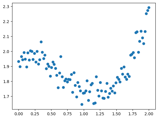
# Dataset creation with du "normal" noise
x = np.linspace(0, 2, 100)
y = 1/3*x**3 - 3/5 * x**2 + 2 + np.random.randn(x.shape[0])/20
plt.scatter(x, y)

<matplotlib.collections.PathCollection at 0x7f3bc8b42580>

# Definition of a statistical model 
def f (x, a, b, c, d):
    return a * x**3 + b * x**2 + c * x + d

from scipy import optimize

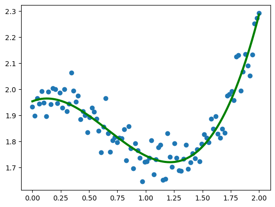
# curve_fit allows to find the parameters of the model f with the least squares method
params, param_cov = optimize.curve_fit(f, x, y)

# Result Visualisation
plt.scatter(x, y)
plt.plot(x, f(x, params[0], params[1], params[2], params[3]), c='g', lw=3)

[<matplotlib.lines.Line2D at 0x7f3bc8331eb0>]

1D minimization

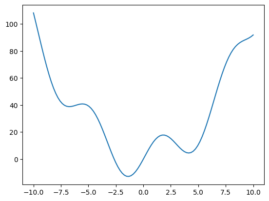
the optimize.minimize function is useful for finding a local minimum in an N-dimensional function

# Definition of a 1 Dimensional function
def f (x):
    return x**2 + 15*np.sin(x)

# Visualisation of the fonction
x = np.linspace(-10, 10, 100)
plt.plot(x, f(x))

[<matplotlib.lines.Line2D at 0x7f3bc82a9a00>]

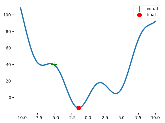
# Definition of a starting point x0 for the minimisation algorithm
x0=-5
result = optimize.minimize(f, x0=x0).x # minimisation result

plt.plot(x, f(x), lw=3, zorder=-1) # the function curve
plt.scatter(x0, f(x0), s=200, marker='+', c='g', zorder=1, label='initial') # initial point 
plt.scatter(result, f(result), s=100, c='r', zorder=1, label='final') # final point
plt.legend()
plt.show()

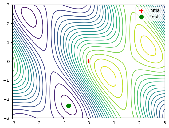
Minimisation 2D

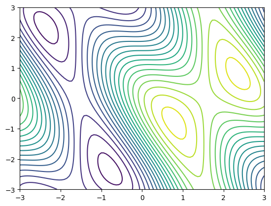
# Definition of 2D function. X is a numpy 2-Dimensional ndarray
def f (x):
    return np.sin(x[0]) + np.cos(x[0]+x[1])*np.cos(x[0])

# Generation of the function over a 2D space.
x = np.linspace(-3, 3, 100)
y = np.linspace(-3, 3, 100)
x, y = np.meshgrid(x, y)

plt.contour(x, y, f(np.array([x, y])), 20)

<matplotlib.contour.QuadContourSet at 0x7f3bc81ab340>

# Setting the initial point x0 at (0,0)
x0 = np.zeros((2, 1))

# Function Minimisation
result = optimize.minimize(f, x0=x0).x
print('The minimum is at coordinates', result) # print the result 

# Visualisation du résultat
plt.contour(x, y, f(np.array([x, y])), 20) # 2D function
plt.scatter(x0[0], x0[1], marker='+', c='r', s=100, label='initial') # initial point
plt.scatter(result[0], result[1], c='g', s=100, label='final') # final point
plt.legend()
plt.show()

The minimum is at coordinates [-0.78539916 -2.35619344]

/tmp/ipykernel_3878359/2502038826.py:5: DeprecationWarning: Use of `minimize` with `x0.ndim != 1` is deprecated. Currently, singleton dimensions will be removed from `x0`, but an error will be raised in SciPy 1.11.0.
  result = optimize.minimize(f, x0=x0).x

3) Signal processing

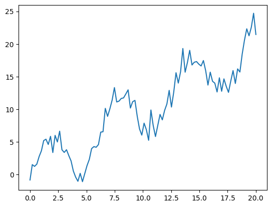
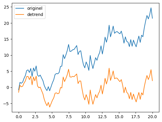
The scipy.signal module contains a lot of convolution functions and filters for signal processing. The signal.detrend function is perfect for eliminating a linear trend in a signal. Useful for many applications!

The scipy.fftpack module contains very powerful and easy-to-use functions to perform Fourier transforms

# Dataset Creation with linear drift 
x = np.linspace(0, 20, 100)
y = x + 4*np.sin(x) +np.random.randn(x.shape[0])
plt.plot(x, y)

[<matplotlib.lines.Line2D at 0x7f3bc660f6a0>]

from scipy import signal

# Elimination of the linear trend
new_y = signal.detrend(y)

# Visualization of results
plt.plot(x, y, label='originel')
plt.plot(x, new_y, label='detrend')
plt.legend()
plt.show()

Fourier transform (FFT)

The Fourier transform is a powerful mathematical technique and normally complex to implement. Fortunately scipy.fftpack makes this technique very simple to implement

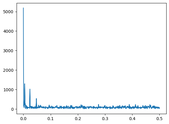
The Fourier transform makes it possible to analyze the frequencies that make up a periodic signal (which repeats over time). This produces a graph called Spectre.

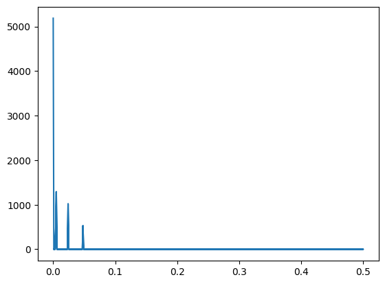
Once the Spectrum is generated, it is possible to filter unwanted noise, or to select only certain frequencies, or to attenuate others… The possibilities are endless.

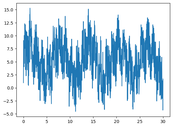
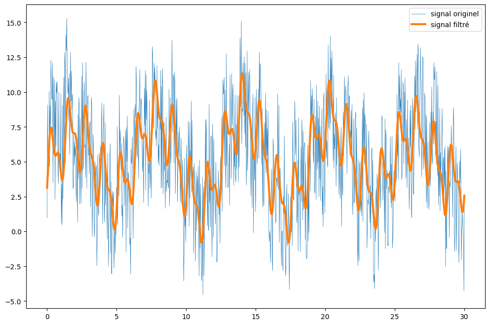
In the example below, we see how to filter out a signal drowned in noise.

# Création d'un signal périodique noyé dans du bruit.
x = np.linspace(0, 30, 1000)
y = 3*np.sin(x) + 2*np.sin(5*x) + np.sin(10*x) + np.random.random(x.shape[0])*10
plt.plot(x, y)

[<matplotlib.lines.Line2D at 0x7f3bc560e7c0>]

from scipy import fftpack

# Creation of a periodic signal embedded in noise.
fourier = fftpack.fft(y)
power = np.abs(fourier) # the power variable is created to eliminate negative amplitudes
frequences = fftpack.fftfreq(y.size)
plt.plot(np.abs(frequences), power)

[<matplotlib.lines.Line2D at 0x7f3bc555a220>]

# spectrum filter with Numpy boolean indexing
fourier[power<400] = 0

# Visualization of the clean speter
plt.plot(np.abs(frequences), np.abs(fourier))

[<matplotlib.lines.Line2D at 0x7f3bc5534be0>]

# Inverse Fourier Transform: generates a new time signal from the filtered spectrum
filtered_signal = fftpack.ifft(fourier)

# Viewing the results

plt.figure(figsize=(12, 8))
plt.plot(x, y, lw=0.5, label='signal originel')
plt.plot(x, filtered_signal, lw=3, label='signal filtré')
plt.legend()
plt.show()

/home/ubuntu/Documents/Projects/msci_data/.venv/lib/python3.9/site-packages/matplotlib/cbook/__init__.py:1298: ComplexWarning: Casting complex values to real discards the imaginary part
  return np.asarray(x, float)

4) Image processing

scipy.ndimage offers many actions for image processing: convolutions, Gaussian filters, measurement method, and morphology.

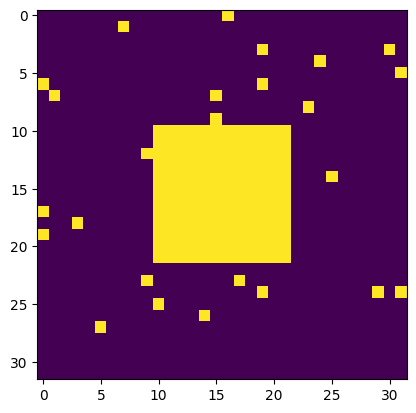
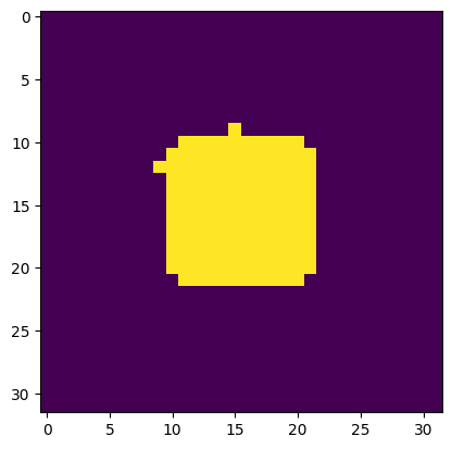
Morphology is a technique that transforms a matrix (and therefore an image) by moving a structure on each pixel of the image. When a “white” pixel is visited, the structure can perform an operation:

expansion: prints pixels

erosion: erases pixels

This technique can be useful to clean an image of artifacts that can compose it.

from scipy import ndimage

np.random.seed(0)
X = np.zeros((32, 32))
X[10:-10, 10:-10] = 1
X[np.random.randint(0,32,30),np.random.randint(0,32,30)] = 1 #ajout d'artefacts aléatoires
plt.imshow(X)

<matplotlib.image.AxesImage at 0x7f3bc54074f0>

# binary_opening operation = erosion then dilation
open_X = ndimage.binary_opening(X)
plt.imshow(open_X)

<matplotlib.image.AxesImage at 0x7f3bc53e1ca0>

5) Application: Image processing (real case)

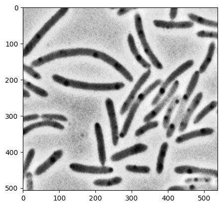
You can download this image at:

# import pyplot image
image = plt.imread('../data/bacteria.png')
image = image[:,:,0] # reduce the image to 2D
plt.imshow(image, cmap='gray') # show image
image.shape

(507, 537)

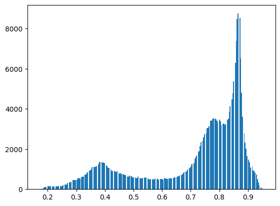
# copy the image, then create the histogram
image_2 = np.copy(image)
plt.hist(image_2.ravel(), bins=255)
plt.show()

# boolean indexing: creation of the binary image
image= image<0.6
plt.imshow(image)

<matplotlib.image.AxesImage at 0x7f3bc54f5f40>

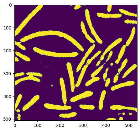
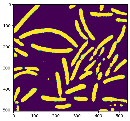
# morphologie utilisée pour enlever les artefacts
open_image = ndimage.binary_opening(image)
plt.imshow(open_image)

<matplotlib.image.AxesImage at 0x7f3bc56a7ca0>

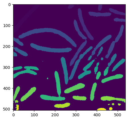
# image Segmentation: label_image contians the different labels and n_labels is the number of unique labels
label_image, n_labels = ndimage.label(open_image)
print(f'il y a {n_labels} groupes')

il y a 53 groupes

# Visualisation of the image after labelisation 
plt.imshow(label_image)

<matplotlib.image.AxesImage at 0x7f3bc5346ca0>

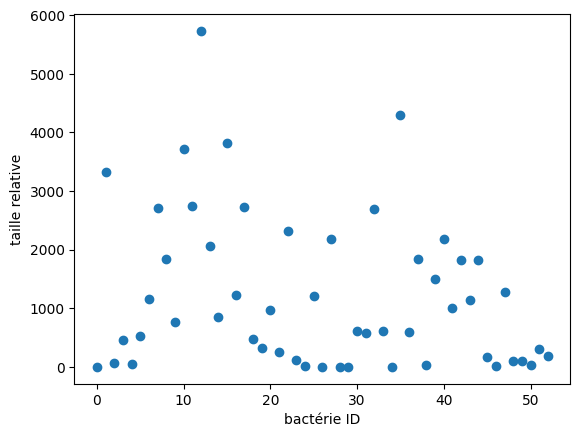
# Mesure de la taille de chaque groupes de label_images (fait la somme des pixels)
sizes = ndimage.sum(open_image, label_image, range(n_labels))

# result viewing
plt.scatter(range(n_labels), sizes)
plt.xlabel('bactérie ID')
plt.ylabel('taille relative')
plt.show()