import pandas as pd
import numpy as np
import matplotlib.pyplot as plt
from datetime import datetime
from datetime import timedelta
from pandas.plotting import register_matplotlib_converters
from statsmodels.tsa.stattools import acf, pacf
from statsmodels.tsa.statespace.sarimax import SARIMAX
register_matplotlib_converters()
from time import time
import os
data_folder = '../data/'
9: SARIMA Model#
def parser(s):
    return datetime.strptime(s, '%Y-%m-%d')
#Catfish Sales Data
catfish_sales = pd.read_csv(os.path.join(data_folder, 'catfish.csv'),
                            parse_dates=['Date'], index_col='Date'
                            )
catfish_sales.head()
| Total | |
|---|---|
| Date | |
| 1986-01-01 | 9034 |
| 1986-02-01 | 9596 |
| 1986-03-01 | 10558 |
| 1986-04-01 | 9002 |
| 1986-05-01 | 9239 |
#infer the frequency of the data
catfish_sales = catfish_sales.asfreq(pd.infer_freq(catfish_sales.index))
start_date = datetime(1996,1,1)
end_date = datetime(2000,1,1)
lim_catfish_sales = catfish_sales[start_date:end_date]
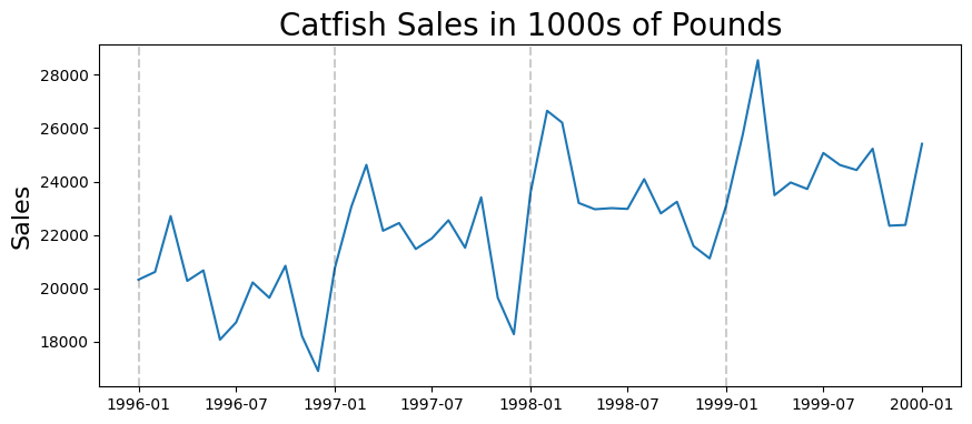
plt.figure(figsize=(10,4))
plt.plot(lim_catfish_sales)
plt.title('Catfish Sales in 1000s of Pounds', fontsize=20)
plt.ylabel('Sales', fontsize=16)
for year in range(start_date.year,end_date.year):
    plt.axvline(pd.to_datetime(str(year)+'-01-01'), color='k', linestyle='--', alpha=0.2)
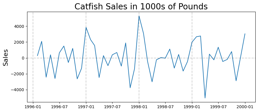
Remove the trend#
first_diff = lim_catfish_sales.diff()[1:]
plt.figure(figsize=(10,4))
plt.plot(first_diff)
plt.title('Catfish Sales in 1000s of Pounds', fontsize=20)
plt.ylabel('Sales', fontsize=16)
for year in range(start_date.year,end_date.year):
    plt.axvline(pd.to_datetime(str(year)+'-01-01'), color='k', linestyle='--', alpha=0.2)
plt.axhline(0, color='k', linestyle='--', alpha=0.2)
<matplotlib.lines.Line2D at 0x7fbb14843af0>
ACF#
acf_vals = acf(first_diff)
num_lags = min(20, len(acf_vals))
plt.bar(range(num_lags), acf_vals[:num_lags])
<BarContainer object of 17 artists>
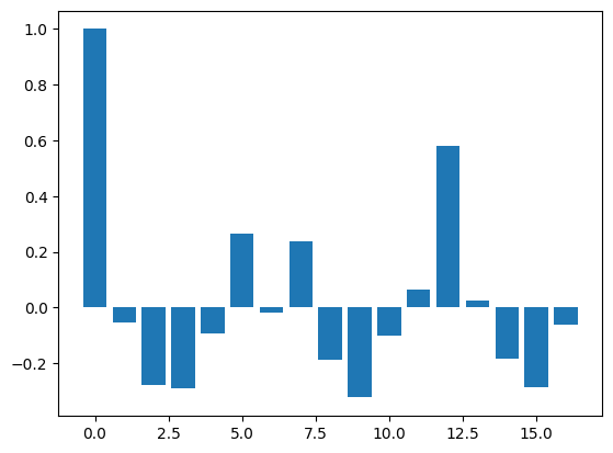
Based on ACF, we should start with a seasonal MA process#
PACF#
pacf_vals = pacf(first_diff)
num_lags = 15
plt.bar(range(num_lags), pacf_vals[:num_lags])
<BarContainer object of 15 artists>
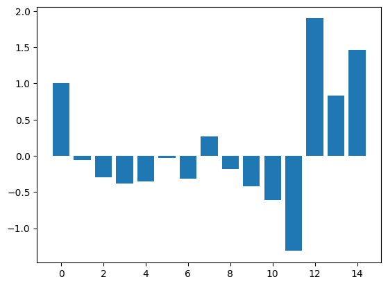
Based on PACF, we should start with a seasonal AR process#
Get training and testing sets#
train_end = datetime(1999,7,1)
test_end = datetime(2000,1,1)

train_data = lim_catfish_sales[:train_end]
test_data = lim_catfish_sales[train_end + timedelta(days=1):test_end]
Fit the SARIMA Model#
my_order = (0,1,0)
my_seasonal_order = (1, 0, 1, 12)
# define model
model = SARIMAX(train_data, order=my_order, seasonal_order=my_seasonal_order)
#fit the model
start = time()
model_fit = model.fit()
end = time()
print('Model Fitting Time:', end - start)
/home/ubuntu/Documents/Projects/STI_FX_Intervention/.venv/lib/python3.9/site-packages/statsmodels/tsa/statespace/sarimax.py:997: UserWarning: Non-stationary starting seasonal autoregressive Using zeros as starting parameters.
  warn('Non-stationary starting seasonal autoregressive'
/home/ubuntu/Documents/Projects/STI_FX_Intervention/.venv/lib/python3.9/site-packages/statsmodels/tsa/statespace/sarimax.py:1009: UserWarning: Non-invertible starting seasonal moving average Using zeros as starting parameters.
  warn('Non-invertible starting seasonal moving average'
 This problem is unconstrained.
RUNNING THE L-BFGS-B CODE

           * * *

Machine precision = 2.220D-16
 N =            3     M =           10

At X0         0 variables are exactly at the bounds

At iterate    0    f=  8.87298D+00    |proj g|=  1.21940D+00

At iterate    5    f=  8.58382D+00    |proj g|=  3.02862D-01

At iterate   10    f=  8.55722D+00    |proj g|=  1.37619D-03

At iterate   15    f=  8.55722D+00    |proj g|=  1.04073D-03

At iterate   20    f=  8.55706D+00    |proj g|=  2.63664D-02

At iterate   25    f=  8.53842D+00    |proj g|=  1.19055D-01

At iterate   30    f=  8.50954D+00    |proj g|=  1.09968D-01

At iterate   35    f=  8.50313D+00    |proj g|=  6.47363D-05

           * * *

Tit   = total number of iterations
Tnf   = total number of function evaluations
Tnint = total number of segments explored during Cauchy searches
Skip  = number of BFGS updates skipped
Nact  = number of active bounds at final generalized Cauchy point
Projg = norm of the final projected gradient
F     = final function value

           * * *

   N    Tit     Tnf  Tnint  Skip  Nact     Projg        F
    3     36     42      1     0     0   9.890D-06   8.503D+00
  F =   8.5031324794697483

CONVERGENCE: NORM_OF_PROJECTED_GRADIENT_<=_PGTOL
Model Fitting Time: 0.39024806022644043
#summary of the model
print(model_fit.summary())
                                      SARIMAX Results
============================================================================================
Dep. Variable:                                Total   No. Observations:                   43
Model:             SARIMAX(0, 1, 0)x(1, 0, [1], 12)   Log Likelihood                -365.635
Date:                              Wed, 22 Mar 2023   AIC                            737.269
Time:                                      13:04:46   BIC                            742.482
Sample:                                  01-01-1996   HQIC                           739.180
                                       - 07-01-1999
Covariance Type:                                opg
==============================================================================
                 coef    std err          z      P>|z|      [0.025      0.975]
------------------------------------------------------------------------------
ar.S.L12       0.8250      0.120      6.848      0.000       0.589       1.061
ma.S.L12      -0.5187      0.197     -2.632      0.008      -0.905      -0.132
sigma2       1.78e+06    4.7e+05      3.791      0.000     8.6e+05     2.7e+06
===================================================================================
Ljung-Box (L1) (Q):                   2.82   Jarque-Bera (JB):                 1.13
Prob(Q):                              0.09   Prob(JB):                         0.57
Heteroskedasticity (H):               0.81   Skew:                            -0.30
Prob(H) (two-sided):                  0.70   Kurtosis:                         2.46
===================================================================================

Warnings:
[1] Covariance matrix calculated using the outer product of gradients (complex-step).
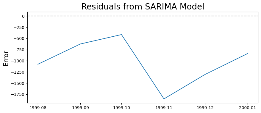
#get the predictions and residuals
predictions = model_fit.forecast(len(test_data))
predictions = pd.Series(predictions, index=test_data.index)
residuals = test_data.squeeze() - predictions.squeeze()
plt.figure(figsize=(10,4))
plt.plot(residuals)
plt.axhline(0, linestyle='--', color='k')
plt.title('Residuals from SARIMA Model', fontsize=20)
plt.ylabel('Error', fontsize=16)
Text(0, 0.5, 'Error')
plt.figure(figsize=(10,4))

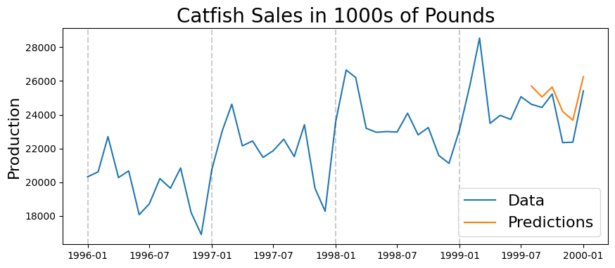
plt.plot(lim_catfish_sales)
plt.plot(predictions)

plt.legend(('Data', 'Predictions'), fontsize=16)

plt.title('Catfish Sales in 1000s of Pounds', fontsize=20)
plt.ylabel('Production', fontsize=16)
for year in range(start_date.year,end_date.year):
    plt.axvline(pd.to_datetime(str(year)+'-01-01'), color='k', linestyle='--', alpha=0.2)
test_data\
    .shape
(6, 1)
print('Mean Absolute Percent Error:', round(np.mean(abs(residuals/test_data.squeeze())),4))
Mean Absolute Percent Error: 0.0433
print('Root Mean Squared Error:', np.sqrt(np.mean(residuals**2)))
Root Mean Squared Error: 1122.3056943982156
Using the Rolling Forecast Origin#
rolling_predictions = test_data.squeeze().copy()
for train_end in test_data.index:
    train_data = lim_catfish_sales[:train_end-timedelta(days=1)]
    model = SARIMAX(train_data, order=my_order, seasonal_order=my_seasonal_order)
    model_fit = model.fit()

    pred = model_fit.forecast()
    rolling_predictions[train_end] = pred
/home/ubuntu/Documents/Projects/STI_FX_Intervention/.venv/lib/python3.9/site-packages/statsmodels/tsa/statespace/sarimax.py:997: UserWarning: Non-stationary starting seasonal autoregressive Using zeros as starting parameters.
  warn('Non-stationary starting seasonal autoregressive'
/home/ubuntu/Documents/Projects/STI_FX_Intervention/.venv/lib/python3.9/site-packages/statsmodels/tsa/statespace/sarimax.py:1009: UserWarning: Non-invertible starting seasonal moving average Using zeros as starting parameters.
  warn('Non-invertible starting seasonal moving average'
 This problem is unconstrained.
RUNNING THE L-BFGS-B CODE

           * * *

Machine precision = 2.220D-16
 N =            3     M =           10

At X0         0 variables are exactly at the bounds

At iterate    0    f=  8.87298D+00    |proj g|=  1.21940D+00

At iterate    5    f=  8.58382D+00    |proj g|=  3.02862D-01

At iterate   10    f=  8.55722D+00    |proj g|=  1.37619D-03

At iterate   15    f=  8.55722D+00    |proj g|=  1.04073D-03

At iterate   20    f=  8.55706D+00    |proj g|=  2.63664D-02

At iterate   25    f=  8.53842D+00    |proj g|=  1.19055D-01

At iterate   30    f=  8.50954D+00    |proj g|=  1.09968D-01

At iterate   35    f=  8.50313D+00    |proj g|=  6.47363D-05

           * * *

Tit   = total number of iterations
Tnf   = total number of function evaluations
Tnint = total number of segments explored during Cauchy searches
Skip  = number of BFGS updates skipped
Nact  = number of active bounds at final generalized Cauchy point
Projg = norm of the final projected gradient
F     = final function value

           * * *

   N    Tit     Tnf  Tnint  Skip  Nact     Projg        F
    3     36     42      1     0     0   9.890D-06   8.503D+00
  F =   8.5031324794697483

CONVERGENCE: NORM_OF_PROJECTED_GRADIENT_<=_PGTOL
RUNNING THE L-BFGS-B CODE

           * * *

Machine precision = 2.220D-16
 N =            3     M =           10

At X0         0 variables are exactly at the bounds

At iterate    0    f=  8.86146D+00    |proj g|=  1.17851D+00

At iterate    5    f=  8.58541D+00    |proj g|=  2.95359D-01

At iterate   10    f=  8.55888D+00    |proj g|=  1.27378D-03

At iterate   15    f=  8.55887D+00    |proj g|=  1.07237D-03

At iterate   20    f=  8.55865D+00    |proj g|=  2.23676D-02

At iterate   25    f=  8.54422D+00    |proj g|=  9.33866D-02

At iterate   30    f=  8.51628D+00    |proj g|=  6.40516D-03

At iterate   35    f=  8.50320D+00    |proj g|=  5.14638D-02

At iterate   40    f=  8.50171D+00    |proj g|=  3.18832D-04

           * * *

Tit   = total number of iterations
Tnf   = total number of function evaluations
Tnint = total number of segments explored during Cauchy searches
Skip  = number of BFGS updates skipped
Nact  = number of active bounds at final generalized Cauchy point
Projg = norm of the final projected gradient
F     = final function value

           * * *

   N    Tit     Tnf  Tnint  Skip  Nact     Projg        F
    3     42     57      1     0     0   1.150D-05   8.502D+00
  F =   8.5017078608695442

CONVERGENCE: REL_REDUCTION_OF_F_<=_FACTR*EPSMCH
RUNNING THE L-BFGS-B CODE

           * * *

Machine precision = 2.220D-16
 N =            3     M =           10

At X0         0 variables are exactly at the bounds

At iterate    0    f=  8.87333D+00    |proj g|=  1.28467D+00

At iterate    5    f=  8.55730D+00    |proj g|=  2.83954D-01
/home/ubuntu/Documents/Projects/STI_FX_Intervention/.venv/lib/python3.9/site-packages/statsmodels/tsa/statespace/sarimax.py:997: UserWarning: Non-stationary starting seasonal autoregressive Using zeros as starting parameters.
warn('Non-stationary starting seasonal autoregressive'
/home/ubuntu/Documents/Projects/STI_FX_Intervention/.venv/lib/python3.9/site-packages/statsmodels/tsa/statespace/sarimax.py:1009: UserWarning: Non-invertible starting seasonal moving average Using zeros as starting parameters.
warn('Non-invertible starting seasonal moving average'
This problem is unconstrained.
At iterate   10    f=  8.53521D+00    |proj g|=  1.26069D-03

At iterate   15    f=  8.53521D+00    |proj g|=  1.24035D-03

At iterate   20    f=  8.53507D+00    |proj g|=  1.47441D-02

At iterate   25    f=  8.52406D+00    |proj g|=  8.24832D-02

At iterate   30    f=  8.50492D+00    |proj g|=  6.77856D-02

At iterate   35    f=  8.49450D+00    |proj g|=  1.54197D-02

           * * *

Tit   = total number of iterations
Tnf   = total number of function evaluations
Tnint = total number of segments explored during Cauchy searches
Skip  = number of BFGS updates skipped
Nact  = number of active bounds at final generalized Cauchy point
Projg = norm of the final projected gradient
F     = final function value

           * * *

   N    Tit     Tnf  Tnint  Skip  Nact     Projg        F
    3     39     59      1     0     0   1.504D-05   8.494D+00
  F =   8.4942658984964972

CONVERGENCE: REL_REDUCTION_OF_F_<=_FACTR*EPSMCH
RUNNING THE L-BFGS-B CODE

           * * *

Machine precision = 2.220D-16
 N =            3     M =           10

At X0         0 variables are exactly at the bounds

At iterate    0    f=  8.97326D+00    |proj g|=  1.68058D+00

At iterate    5    f=  8.50772D+00    |proj g|=  1.82687D-01

At iterate   10    f=  8.49272D+00    |proj g|=  8.30154D-04

           * * *

Tit   = total number of iterations
Tnf   = total number of function evaluations
Tnint = total number of segments explored during Cauchy searches
Skip  = number of BFGS updates skipped
Nact  = number of active bounds at final generalized Cauchy point
Projg = norm of the final projected gradient
F     = final function value

           * * *

   N    Tit     Tnf  Tnint  Skip  Nact     Projg        F
    3     12     14      1     0     0   9.774D-05   8.493D+00
  F =   8.4927175966901274

CONVERGENCE: REL_REDUCTION_OF_F_<=_FACTR*EPSMCH
RUNNING THE L-BFGS-B CODE

           * * *

Machine precision = 2.220D-16
 N =            3     M =           10

At X0         0 variables are exactly at the bounds

At iterate    0    f=  8.97866D+00    |proj g|=  1.62914D+00
/home/ubuntu/Documents/Projects/STI_FX_Intervention/.venv/lib/python3.9/site-packages/statsmodels/tsa/statespace/sarimax.py:997: UserWarning: Non-stationary starting seasonal autoregressive Using zeros as starting parameters.
warn('Non-stationary starting seasonal autoregressive'
/home/ubuntu/Documents/Projects/STI_FX_Intervention/.venv/lib/python3.9/site-packages/statsmodels/tsa/statespace/sarimax.py:1009: UserWarning: Non-invertible starting seasonal moving average Using zeros as starting parameters.
warn('Non-invertible starting seasonal moving average'
This problem is unconstrained.
At iterate    5    f=  8.52124D+00    |proj g|=  1.34321D-01

At iterate   10    f=  8.50097D+00    |proj g|=  1.43343D-03

At iterate   15    f=  8.50096D+00    |proj g|=  3.70428D-04

At iterate   20    f=  8.50084D+00    |proj g|=  3.94992D-03

At iterate   25    f=  8.49494D+00    |proj g|=  2.13762D-02

At iterate   30    f=  8.48986D+00    |proj g|=  1.55626D-03

           * * *

Tit   = total number of iterations
Tnf   = total number of function evaluations
Tnint = total number of segments explored during Cauchy searches
Skip  = number of BFGS updates skipped
Nact  = number of active bounds at final generalized Cauchy point
Projg = norm of the final projected gradient
F     = final function value

           * * *

   N    Tit     Tnf  Tnint  Skip  Nact     Projg        F
    3     33     38      1     0     0   2.780D-05   8.490D+00
  F =   8.4898467447992996

CONVERGENCE: REL_REDUCTION_OF_F_<=_FACTR*EPSMCH
RUNNING THE L-BFGS-B CODE

           * * *

Machine precision = 2.220D-16
 N =            3     M =           10

At X0         0 variables are exactly at the bounds

At iterate    0    f=  9.50185D+00    |proj g|=  7.44698D-01

At iterate    5    f=  8.51191D+00    |proj g|=  5.91494D-04

At iterate   10    f=  8.50176D+00    |proj g|=  1.05432D-01

At iterate   15    f=  8.48764D+00    |proj g|=  1.00690D-02

           * * *

Tit   = total number of iterations
Tnf   = total number of function evaluations
Tnint = total number of segments explored during Cauchy searches
Skip  = number of BFGS updates skipped
Nact  = number of active bounds at final generalized Cauchy point
Projg = norm of the final projected gradient
F     = final function value

           * * *

   N    Tit     Tnf  Tnint  Skip  Nact     Projg        F
    3     18     42      1     0     0   8.047D-05   8.488D+00
  F =   8.4876232442262598

CONVERGENCE: REL_REDUCTION_OF_F_<=_FACTR*EPSMCH
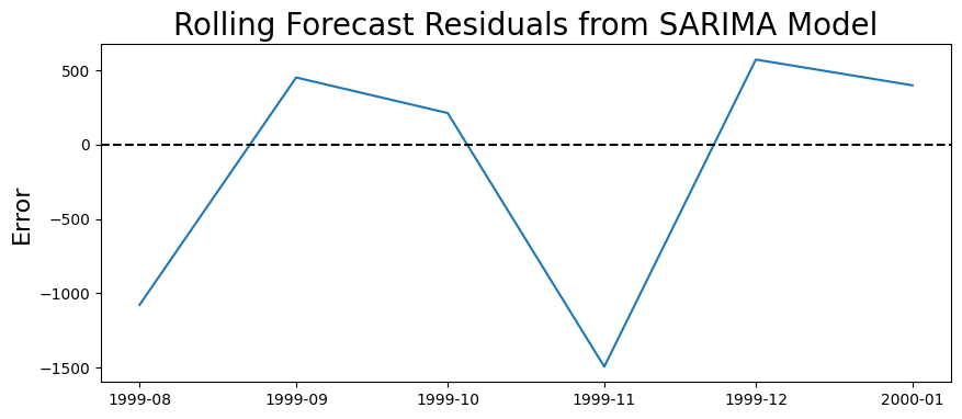
rolling_residuals = test_data.squeeze() - rolling_predictions.squeeze()
plt.figure(figsize=(10,4))
plt.plot(rolling_residuals)
plt.axhline(0, linestyle='--', color='k')
plt.title('Rolling Forecast Residuals from SARIMA Model', fontsize=20)
plt.ylabel('Error', fontsize=16)
Text(0, 0.5, 'Error')
plt.figure(figsize=(10,4))

plt.plot(lim_catfish_sales)
plt.plot(rolling_predictions)

plt.legend(('Data', 'Predictions'), fontsize=16)

plt.title('Catfish Sales in 1000s of Pounds', fontsize=20)
plt.ylabel('Production', fontsize=16)
for year in range(start_date.year,end_date.year):
    plt.axvline(pd.to_datetime(str(year)+'-01-01'), color='k', linestyle='--', alpha=0.2)
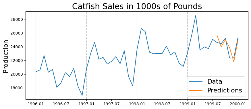
print('Mean Absolute Percent Error:', round(np.mean(abs(rolling_residuals/test_data.squeeze())),4))
Mean Absolute Percent Error: 0.0298
print('Root Mean Squared Error:', np.sqrt(np.mean(rolling_residuals**2)))
Root Mean Squared Error: 829.3411406660159

