![]()
17: Pandas (the Basics) and Titanic Analysis#
import numpy as np
import matplotlib.pyplot as plt
import pandas as pd
1. Load your data into a Pandas DataFrame#
The most common options:
read_csv
read_excel
data = pd.read_excel('../data/titanic3 (3).xls')
data.shape
data.head()
| pclass | survived | name | sex | age | sibsp | parch | ticket | fare | cabin | embarked | boat | body | home.dest | |
|---|---|---|---|---|---|---|---|---|---|---|---|---|---|---|
| 0 | 1 | 1 | Allen, Miss. Elisabeth Walton | female | 29.0000 | 0 | 0 | 24160 | 211.3375 | B5 | S | 2 | NaN | St Louis, MO |
| 1 | 1 | 1 | Allison, Master. Hudson Trevor | male | 0.9167 | 1 | 2 | 113781 | 151.5500 | C22 C26 | S | 11 | NaN | Montreal, PQ / Chesterville, ON |
| 2 | 1 | 0 | Allison, Miss. Helen Loraine | female | 2.0000 | 1 | 2 | 113781 | 151.5500 | C22 C26 | S | NaN | NaN | Montreal, PQ / Chesterville, ON |
| 3 | 1 | 0 | Allison, Mr. Hudson Joshua Creighton | male | 30.0000 | 1 | 2 | 113781 | 151.5500 | C22 C26 | S | NaN | 135.0 | Montreal, PQ / Chesterville, ON |
| 4 | 1 | 0 | Allison, Mrs. Hudson J C (Bessie Waldo Daniels) | female | 25.0000 | 1 | 2 | 113781 | 151.5500 | C22 C26 | S | NaN | NaN | Montreal, PQ / Chesterville, ON |
data.describe()
| pclass | survived | age | sibsp | parch | fare | body | |
|---|---|---|---|---|---|---|---|
| count | 1309.000000 | 1309.000000 | 1046.000000 | 1309.000000 | 1309.000000 | 1308.000000 | 121.000000 |
| mean | 2.294882 | 0.381971 | 29.881135 | 0.498854 | 0.385027 | 33.295479 | 160.809917 |
| std | 0.837836 | 0.486055 | 14.413500 | 1.041658 | 0.865560 | 51.758668 | 97.696922 |
| min | 1.000000 | 0.000000 | 0.166700 | 0.000000 | 0.000000 | 0.000000 | 1.000000 |
| 25% | 2.000000 | 0.000000 | 21.000000 | 0.000000 | 0.000000 | 7.895800 | 72.000000 |
| 50% | 3.000000 | 0.000000 | 28.000000 | 0.000000 | 0.000000 | 14.454200 | 155.000000 |
| 75% | 3.000000 | 1.000000 | 39.000000 | 1.000000 | 0.000000 | 31.275000 | 256.000000 |
| max | 3.000000 | 1.000000 | 80.000000 | 8.000000 | 9.000000 | 512.329200 | 328.000000 |
2. Clean up your dataset with drop(), dropna() and fillna()#
data = data.drop(['name', 'sibsp', 'parch', 'ticket', 'fare', 'cabin', 'embarked', 'boat', 'body', 'home.dest'], axis=1)
data = data.dropna(axis=0)
data.shape
(1046, 4)
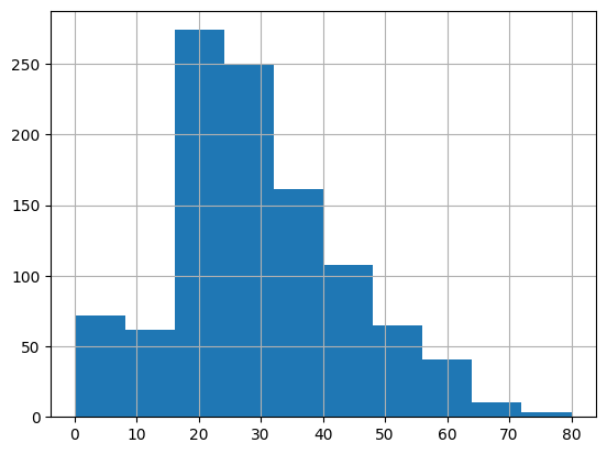
data['age'].hist()
<Axes: >
3. Groupby() and value_counts()#
data.groupby(['sex']).mean()
| pclass | survived | age | |
|---|---|---|---|
| sex | |||
| female | 2.048969 | 0.752577 | 28.687071 |
| male | 2.300912 | 0.205167 | 30.585233 |
data.groupby(['sex', 'pclass']).mean()
| survived | age | ||
|---|---|---|---|
| sex | pclass | ||
| female | 1 | 0.962406 | 37.037594 |
| 2 | 0.893204 | 27.499191 | |
| 3 | 0.473684 | 22.185307 | |
| male | 1 | 0.350993 | 41.029250 |
| 2 | 0.145570 | 30.815401 | |
| 3 | 0.169054 | 25.962273 |
data['pclass'].value_counts()
3    501
1    284
2    261
Name: pclass, dtype: int64
data[data['age'] < 18]['pclass'].value_counts()
3    106
2     33
1     15
Name: pclass, dtype: int64
4. Exercice#
Créer des catégories d’ages avec la fonction map() de pandas
Créer des catégories de genres avec cat.codes
Solution#
Show code cell content
def category_ages(age):
    if age <= 20:
        return '<20 ans'
    elif (age > 20) & (age <= 30):
        return '20-30 ans'
    elif (age > 30) & (age <= 40):
        return '30-40 ans'
    else:
        return '+40 ans'
Show code cell content
data['age'] = data['age'].map(category_ages)
Show code cell content
data['sex'].astype('category').cat.codes
0       0
1       1
2       0
3       1
4       0
       ..
1301    1
1304    0
1306    1
1307    1
1308    1
Length: 1046, dtype: int8