import matplotlib.pyplot as plt
import numpy as np
from statsmodels.tsa.stattools import adfuller
from statsmodels.graphics.tsaplots import plot_acf, plot_pacf
from statsmodels.tsa.arima.model import ARIMA
import pandas as pd

def perform_adf_test(series):
    result = adfuller(series)
    print('ADF Statistic: %f' % result[0])
    print('p-value: %f' % result[1])

10: Undo Stationarity Transformation

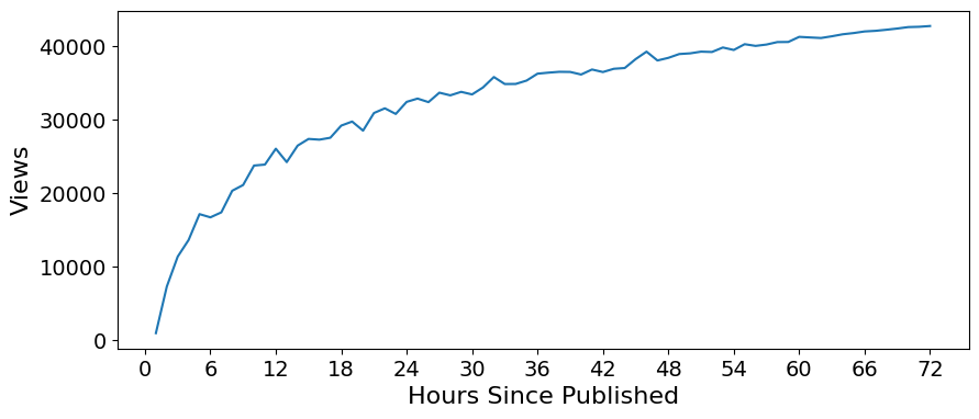
Original Series

ts = pd.read_csv('../data/original_series.csv')
ts.index = np.arange(1,len(ts)+1)

plt.figure(figsize=(10,4))
plt.plot(ts)

plt.xticks(np.arange(0,78,6), fontsize=14)
plt.xlabel('Hours Since Published', fontsize=16)

plt.yticks(np.arange(0,50000,10000), fontsize=14)
plt.ylabel('Views', fontsize=16)

Text(0, 0.5, 'Views')

Original Series: \(v_t\)

1. Normalize (\(v_t \rightarrow n_t\)): \(n_t = \frac{v_t - \mu}{\sigma}\)

2. Exponentiate (\(n_t \rightarrow e_t\)): \(e_t = e^{n_t}\)

3. First Difference (\(e_t \rightarrow d_t\)): \(d_t = e_t - e_{t-1}\)

\(d_t = e^{\frac{v_t - \mu}{\sigma}} - e^{\frac{v_{t-1} - \mu}{\sigma}}\)

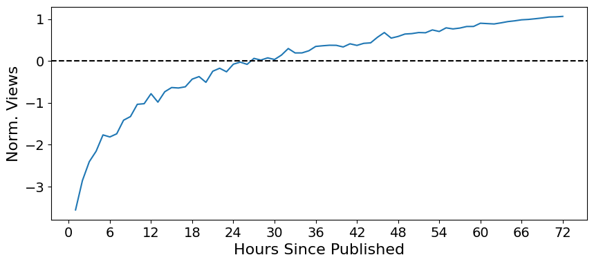
1. Normalize

mu = np.mean(ts).iloc[0]
sigma = np.std(ts).iloc[0]

norm_ts = (ts - mu) / sigma

plt.figure(figsize=(10,4))
plt.plot(norm_ts)

plt.xticks(np.arange(0,78,6), fontsize=14)
plt.xlabel('Hours Since Published', fontsize=16)

plt.yticks(np.arange(-3,2), fontsize=14)
plt.ylabel('Norm. Views', fontsize=16)

plt.axhline(0, color='k', linestyle='--')

<matplotlib.lines.Line2D at 0x7f5c58be18e0>

2. Exponentiate

exp_ts = np.exp(norm_ts)

plt.figure(figsize=(10,4))
plt.plot(exp_ts)

plt.xticks(np.arange(0,78,6), fontsize=14)
plt.xlabel('Hours Since Published', fontsize=16)

plt.yticks(np.arange(0,3.5,.5), fontsize=14)
plt.ylabel('Exp. Norm. Views', fontsize=16)

Text(0, 0.5, 'Exp. Norm. Views')

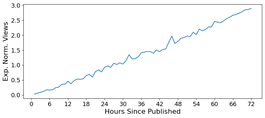
perform_adf_test(exp_ts)

ADF Statistic: 1.648979
p-value: 0.997997

3. First Difference

diff_ts = exp_ts.diff().dropna()

plt.figure(figsize=(10,4))
plt.plot(diff_ts)

plt.xticks(np.arange(0,78,6), fontsize=14)
plt.xlabel('Hours Since Published', fontsize=16)

plt.yticks(np.arange(-0.2,0.3,.1), fontsize=14)
plt.ylabel('First Diff. \nExp. Norm. Views', fontsize=16)

Text(0, 0.5, 'First Diff. \nExp. Norm. Views')

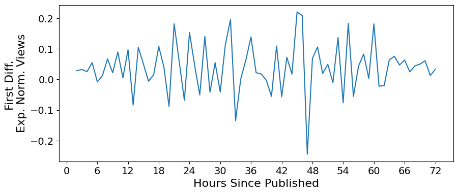
perform_adf_test(diff_ts)

ADF Statistic: -4.881064
p-value: 0.000038

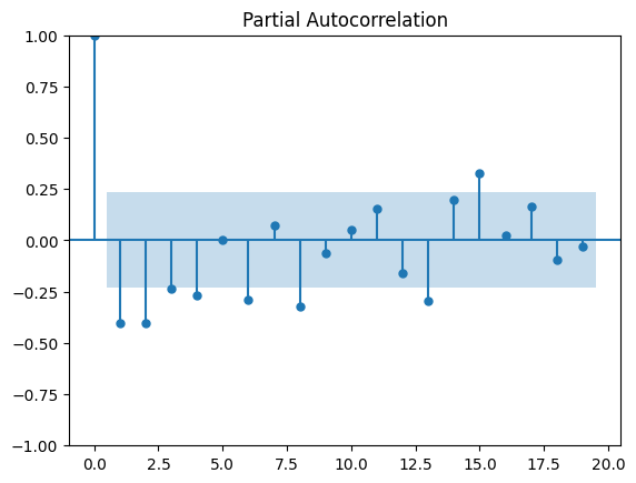
Fit AR Model

plot_pacf(diff_ts)
plt.show()

/home/ubuntu/Documents/Projects/msci_data/.venv/lib/python3.9/site-packages/statsmodels/graphics/tsaplots.py:348: FutureWarning: The default method 'yw' can produce PACF values outside of the [-1,1] interval. After 0.13, the default will change tounadjusted Yule-Walker ('ywm'). You can use this method now by setting method='ywm'.
  warnings.warn(

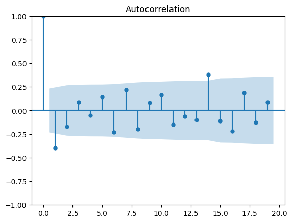
plot_acf(diff_ts)
plt.show()

#create the model
model = ARIMA(diff_ts, order=(4,1,0))

/home/ubuntu/Documents/Projects/msci_data/.venv/lib/python3.9/site-packages/statsmodels/tsa/base/tsa_model.py:471: ValueWarning: An unsupported index was provided and will be ignored when e.g. forecasting.
  self._init_dates(dates, freq)
/home/ubuntu/Documents/Projects/msci_data/.venv/lib/python3.9/site-packages/statsmodels/tsa/base/tsa_model.py:471: ValueWarning: An unsupported index was provided and will be ignored when e.g. forecasting.
  self._init_dates(dates, freq)
/home/ubuntu/Documents/Projects/msci_data/.venv/lib/python3.9/site-packages/statsmodels/tsa/base/tsa_model.py:471: ValueWarning: An unsupported index was provided and will be ignored when e.g. forecasting.
  self._init_dates(dates, freq)

model_fit = model.fit()

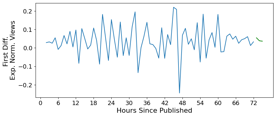
Predict Out 3 Hours

predictions = model_fit.forecast(3)

/home/ubuntu/Documents/Projects/msci_data/.venv/lib/python3.9/site-packages/statsmodels/tsa/base/tsa_model.py:834: ValueWarning: No supported index is available. Prediction results will be given with an integer index beginning at `start`.
  return get_prediction_index(

plt.figure(figsize=(10,4))
plt.plot(diff_ts)

plt.xticks(np.arange(0,78,6), fontsize=14)
plt.xlabel('Hours Since Published', fontsize=16)

plt.yticks(np.arange(-0.2,0.3,.1), fontsize=14)
plt.ylabel('First Diff. \nExp. Norm. Views', fontsize=16)

plt.plot(np.arange(len(ts)+1, len(ts)+4), predictions, color='g')
#plt.fill_between(np.arange(len(ts)+1, len(ts)+4), lower_bound, upper_bound, color='g', alpha=0.1)

[<matplotlib.lines.Line2D at 0x7f5c54ef9e50>]

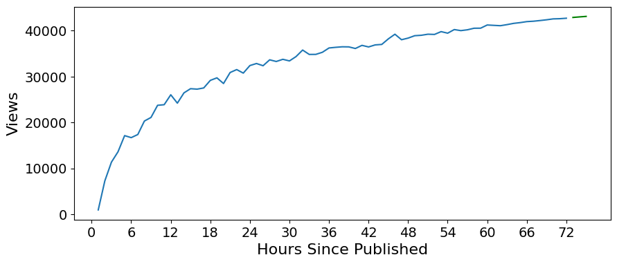
Undo Transformations:

\(\hat{d}_{t+1} \rightarrow \hat{v}_{t+1}\)

\(\hat{v}_{t+1} = \sigma \ln(\hat{d}_{t+1} + e^{\frac{v_t - \mu}{\sigma}}) + \mu\)

def undo_transformations(predictions, series, mu, sigma):
    first_pred = sigma*np.log(predictions.iloc[0] + np.exp((series.iloc[-1]-mu)/sigma)) + mu
    orig_predictions = [first_pred]
    
    for i in range(len(predictions.iloc[1:])):
        next_pred = sigma*np.log(predictions.iloc[i+1] + np.exp((orig_predictions[-1]-mu)/sigma)) + mu
        orig_predictions.append(next_pred)
    
    return np.array(orig_predictions).flatten()

orig_preds = undo_transformations(predictions, ts, mu, sigma)

#orig_lower_bound = undo_transformations(lower_bound, ts, mu, sigma)
#orig_upper_bound = undo_transformations(upper_bound, ts, mu, sigma)

plt.figure(figsize=(10,4))
plt.plot(ts)

plt.xticks(np.arange(0,78,6), fontsize=14)
plt.xlabel('Hours Since Published', fontsize=16)

plt.yticks(np.arange(0,50000,10000), fontsize=14)
plt.ylabel('Views', fontsize=16)

plt.plot(np.arange(len(ts)+1, len(ts)+4), orig_preds, color='g')
#plt.fill_between(np.arange(len(ts)+1, len(ts)+4), orig_lower_bound, orig_upper_bound, color='g', alpha=0.1)

[<matplotlib.lines.Line2D at 0x7f5c54e7cb50>]

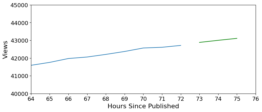
plt.figure(figsize=(10,4))
plt.plot(ts)

plt.xticks(np.arange(0,78), fontsize=14)
plt.xlabel('Hours Since Published', fontsize=16)

plt.yticks(np.arange(40000,46000,1000), fontsize=14)
plt.ylabel('Views', fontsize=16)

plt.plot(np.arange(len(ts)+1, len(ts)+4), orig_preds, color='g')
#plt.fill_between(np.arange(len(ts)+1, len(ts)+4), orig_lower_bound, orig_upper_bound, color='g', alpha=0.1)
plt.xlim(64,76)
plt.ylim(40000, 45000)

(40000.0, 45000.0)