import pandas as pd
import numpy as np
import matplotlib.pyplot as plt
from pandas.plotting import register_matplotlib_converters
from statsmodels.graphics.tsaplots import plot_acf, plot_pacf
from statsmodels.tsa.stattools import acf, pacf
from statsmodels.tsa.arima.model import ARIMA
from datetime import datetime, timedelta
register_matplotlib_converters()
5: Generate Some Data#
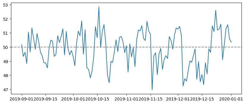
\(y_t = 50 + 0.4\varepsilon_{t-1} + 0.3\varepsilon_{t-2} + \varepsilon_t\)#
\(\varepsilon_t \sim N(0,1)\)#
errors = np.random.normal(0, 1, 400)
date_index = pd.date_range(start='9/1/2019', end='1/1/2020')
mu = 50
series = []
for t in range(1,len(date_index)+1):
    series.append(mu + 0.4*errors[t-1] + 0.3*errors[t-2] + errors[t])
series = pd.Series(series, date_index)
series = series.asfreq(pd.infer_freq(series.index))
plt.figure(figsize=(10,4))
plt.plot(series)
plt.axhline(mu, linestyle='--', color='grey')
<matplotlib.lines.Line2D at 0x7f420c12d400>
def calc_corr(series, lag):
    return pearsonr(series[:-lag], series[lag:])[0]
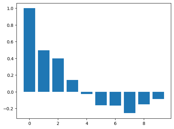
ACF#
acf_vals = acf(series)
num_lags = 10
plt.bar(range(num_lags), acf_vals[:num_lags])
<BarContainer object of 10 artists>
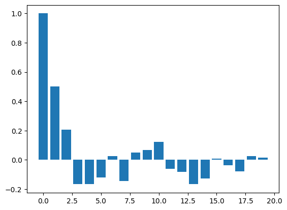
PACF#
pacf_vals = pacf(series)
num_lags = 20
plt.bar(range(num_lags), pacf_vals[:num_lags])
<BarContainer object of 20 artists>
Get training and testing sets#
train_end = datetime(2019,12,30)
test_end = datetime(2020,1,1)

train_data = series[:train_end]
test_data = series[train_end + timedelta(days=1):test_end]
Fit ARIMA Model#
ARIMA?
#create the model
model = ARIMA(train_data, order=(0,0,2))
#fit the model
model_fit = model.fit()
#summary of the model
print(model_fit.summary())
                               SARIMAX Results
==============================================================================
Dep. Variable:                      y   No. Observations:                  121
Model:                 ARIMA(0, 0, 2)   Log Likelihood                -177.787
Date:                Wed, 22 Mar 2023   AIC                            363.575
Time:                        12:58:21   BIC                            374.758
Sample:                    09-01-2019   HQIC                           368.117
                         - 12-30-2019
Covariance Type:                  opg
==============================================================================
                 coef    std err          z      P>|z|      [0.025      0.975]
------------------------------------------------------------------------------
const         49.8920      0.171    292.359      0.000      49.557      50.226
ma.L1          0.3305      0.094      3.498      0.000       0.145       0.516
ma.L2          0.3725      0.088      4.220      0.000       0.199       0.546
sigma2         1.1027      0.143      7.704      0.000       0.822       1.383
===================================================================================
Ljung-Box (L1) (Q):                   0.94   Jarque-Bera (JB):                 4.17
Prob(Q):                              0.33   Prob(JB):                         0.12
Heteroskedasticity (H):               1.77   Skew:                            -0.44
Prob(H) (two-sided):                  0.08   Kurtosis:                         3.20
===================================================================================

Warnings:
[1] Covariance matrix calculated using the outer product of gradients (complex-step).
Predicted Model:#
\(\hat{y}_t = 50 + 0.37\varepsilon_{t-1} + 0.25\varepsilon_{t-2}\)#
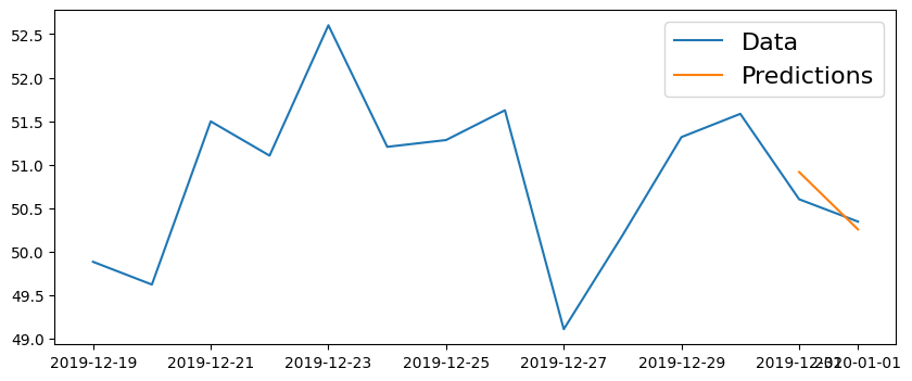
#get prediction start and end dates
pred_start_date = test_data.index[0]
pred_end_date = test_data.index[-1]
#get the predictions and residuals
predictions = model_fit.predict(start=pred_start_date, end=pred_end_date)
residuals = test_data - predictions
plt.figure(figsize=(10,4))

plt.plot(series[-14:])
plt.plot(predictions)

plt.legend(('Data', 'Predictions'), fontsize=16)
<matplotlib.legend.Legend at 0x7f4205f2c580>
print('Mean Absolute Percent Error:', round(np.mean(abs(residuals/test_data)),4))
Mean Absolute Percent Error: 0.004
print('Root Mean Squared Error:', np.sqrt(np.mean(residuals**2)))
Root Mean Squared Error: 0.23016330452025244