import pandas as pd
from statsmodels.tsa.seasonal import STL
import matplotlib.pyplot as plt
from datetime import datetime
import os
data_folder = '../data/'
3: Seasonal-Trend Decomposition using LOESS (STL)#
Read the Data#
ice_cream_interest = pd.read_csv(os.path.join(data_folder, 'ice_cream_interest.csv'))
ice_cream_interest['month'] = pd.to_datetime(ice_cream_interest.month)
ice_cream_interest.set_index('month', inplace=True)
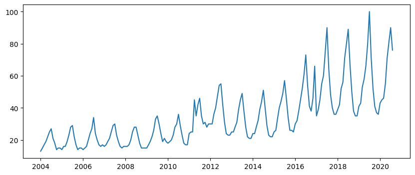
plt.figure(figsize=(10,4))
plt.plot(ice_cream_interest)
[<matplotlib.lines.Line2D at 0x7faa9cc4a580>]
plt.figure(figsize=(10,4))
plt.plot(ice_cream_interest)
for year in range(2004,2021):
    plt.axvline(datetime(year,1,1), color='k', linestyle='--', alpha=0.5)
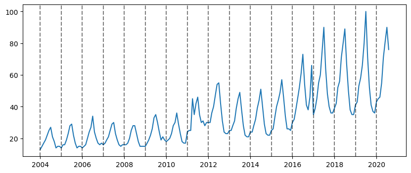
Visual Inspection: Mid-2011 and Late-2016#
Perform STL Decomp#
stl = STL(ice_cream_interest)
result = stl.fit()
seasonal, trend, resid = result.seasonal, result.trend, result.resid
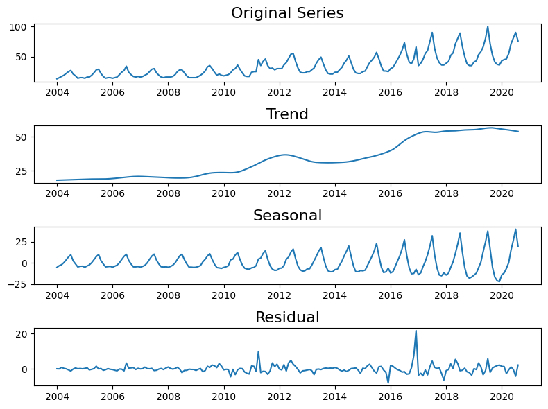
plt.figure(figsize=(8,6))

plt.subplot(4,1,1)
plt.plot(ice_cream_interest)
plt.title('Original Series', fontsize=16)

plt.subplot(4,1,2)
plt.plot(trend)
plt.title('Trend', fontsize=16)

plt.subplot(4,1,3)
plt.plot(seasonal)
plt.title('Seasonal', fontsize=16)

plt.subplot(4,1,4)
plt.plot(resid)
plt.title('Residual', fontsize=16)

plt.tight_layout()
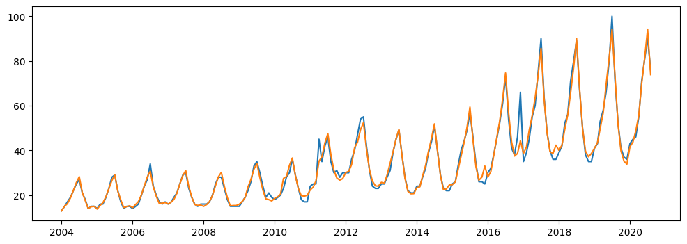
estimated = trend + seasonal
plt.figure(figsize=(12,4))
plt.plot(ice_cream_interest)
plt.plot(estimated)
[<matplotlib.lines.Line2D at 0x7faa9cb6a310>]
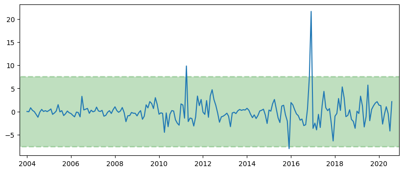
Anomaly Detection#
resid_mu = resid.mean()
resid_dev = resid.std()

lower = resid_mu - 3*resid_dev
upper = resid_mu + 3*resid_dev
plt.figure(figsize=(10,4))
plt.plot(resid)

plt.fill_between([datetime(2003,1,1), datetime(2021,8,1)], lower, upper, color='g', alpha=0.25, linestyle='--', linewidth=2)
plt.xlim(datetime(2003,9,1), datetime(2020,12,1))
(12296.0, 18597.0)
anomalies = ice_cream_interest[(resid < lower) | (resid > upper)]
plt.figure(figsize=(10,4))
plt.plot(ice_cream_interest)
for year in range(2004,2021):
    plt.axvline(datetime(year,1,1), color='k', linestyle='--', alpha=0.5)

plt.scatter(anomalies.index, anomalies.interest, color='r', marker='D')
<matplotlib.collections.PathCollection at 0x7faa9d44e190>
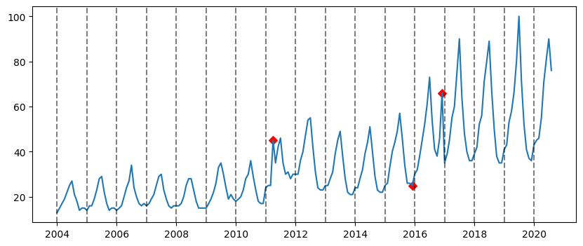
anomalies
| interest | |
|---|---|
| month | |
| 2011-04-01 | 45 |
| 2015-12-01 | 25 |
| 2016-12-01 | 66 |